Dense Fog advisories were issued by the National Weather Service in Grand Forks as visibilities in the WFO dropped to near zero. How did the IFR Probability Fields and traditional Brightness Temperature Difference Fields capture this event? The animation below shows the brightness temperature difference field (10.7 µm – 3.9 µm) from GOES-13. Initially, a swath of mid-level and upper-level clouds covered the Red River Valley (this system had produced very light rains on Monday the 27th), but the clouds moved east and dense fog quickly developed (Cavalier, ND, for example, showed reduced visibility already at 0400 UTC).
GOES-13 Brightness Temperature Difference (10.7 µm – 3.9 µm) hourly from 0315 to 1115 UTC on 28 April 2015, along with surface plots of ceilings and visibility (Click to enlarge)
The IFR Probability fields for the same time, below, better capture the horizontal extent of the fog. For example, the strong signal in the Brightness Temperature Difference field over South Dakota at the end of the animation, above, is not present in the IFR Probability fields. IFR Conditions are not occurring over South Dakota. The good match between the developing IFR Probability fields and the developing fog testifies to the satellite view of the fog and the accurate simulation of this event by the Rapid Refresh model.
GOES-R IFR Probability Fields hourly from 0315 to 1115 UTC on 28 April 2015, along with surface plots of ceilings and visibility (Click to enlarge)
Geostationary GOES fields give good temporal resolution to the evolving field. Polar orbiting satellites, such as Suomi NPP (carrying the VIIRS instrument) and Terra/Aqua (each carrying MODIS) each gave snapshot views of the developing fog. At 0355, IFR Probabilities are low, and the Red River valley is mostly obscured by higher clouds. Four hours later, at 0805 UTC, dense fog has developed and IFR probabilities are large.
Terra MODIS Brightness Temperature Difference (11µm – 3.9µm) and IFR Probability fields, ~0355 UTC on 28 April 2015 (Click to enlarge)
Aqua MODIS Brightness Temperature Difference (11µm – 3.9µm) and IFR Probability fields, ~0805 UTC on 28 April 2015 (Click to enlarge)
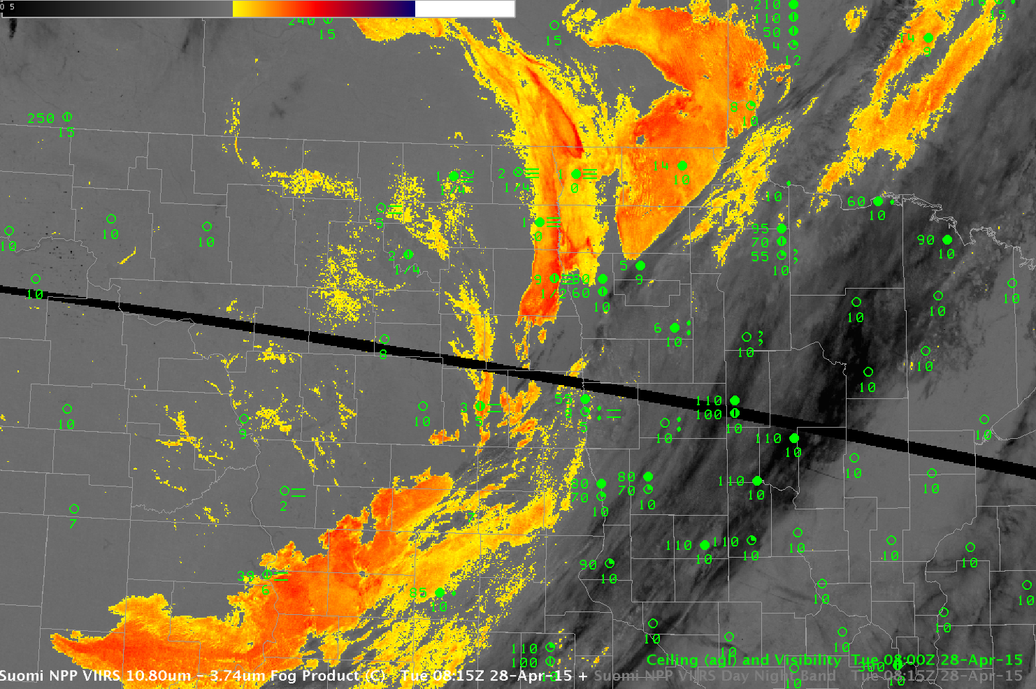
Suomi NPP also viewed the fog field. The toggle between the Day Night Band and the Brightness Temperature Difference field (11.45µm – 3.74µm), below, shows evidence of fog in the visible Day Night band imagery. The lights of western North Dakota’s oil shale fields are also evident.
Polar-orbiting satellites give excellent high-resolution imagery of fog fields. When used in concert with the excellent time resolution of GOES imagery, a complete picture of the evolving fog field can be drawn.
Toggle between Day Night Band (0.70 µm) and Brightness Temperature Difference (11.45µm – 3.74µm) field from VIIRS on Suomi NPP at 0815 UTC (Click to enlarge)