Category Archives: Cloud Thickness

Advection fog over Lake Michigan

GOES_IFR_PROB_20140429loop

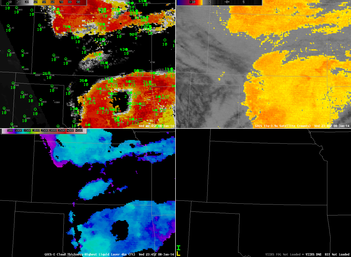
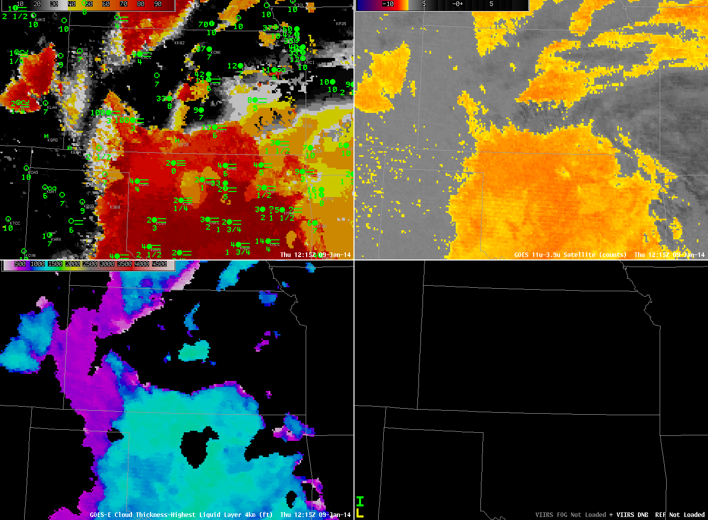
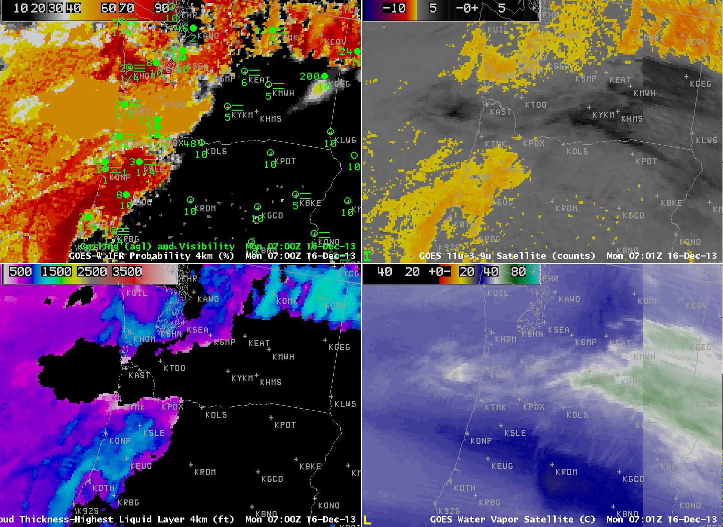
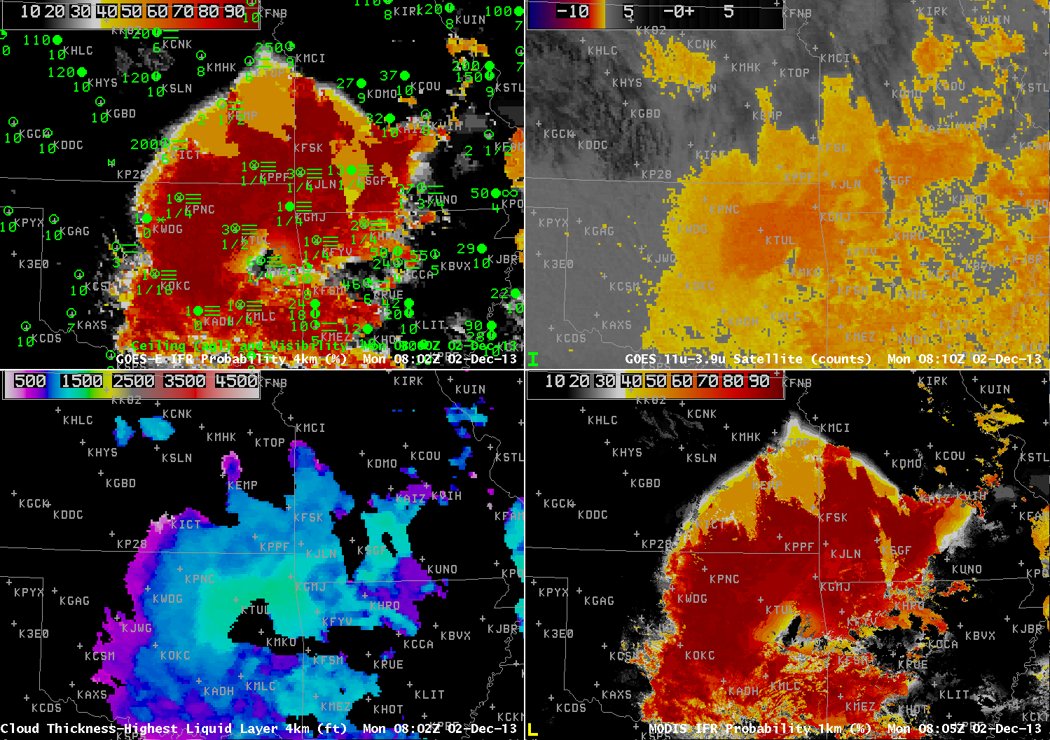
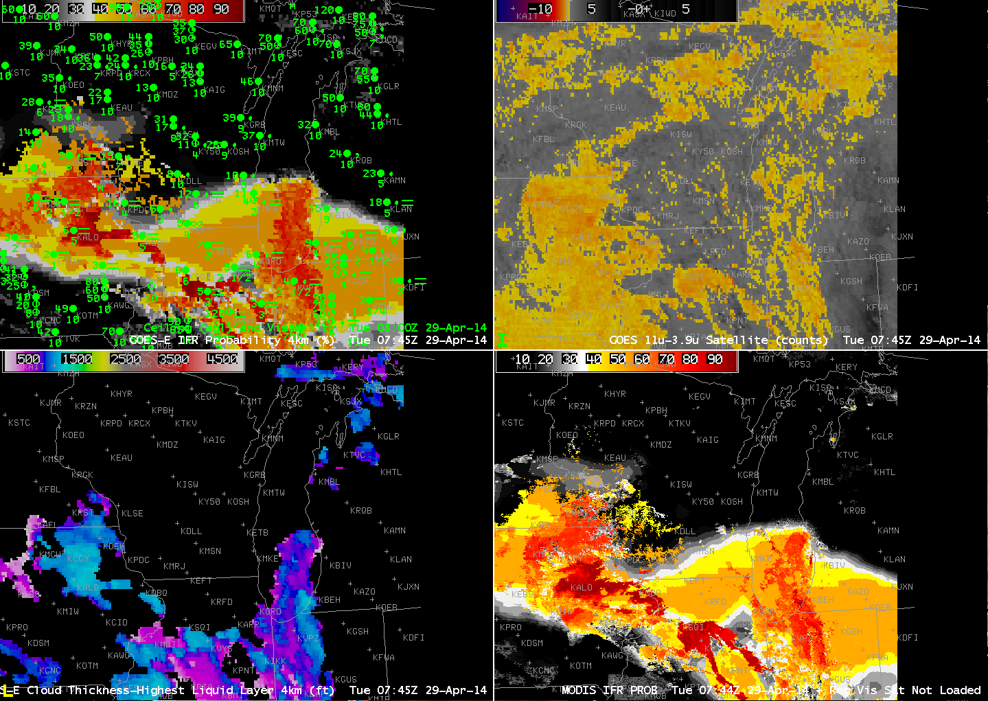
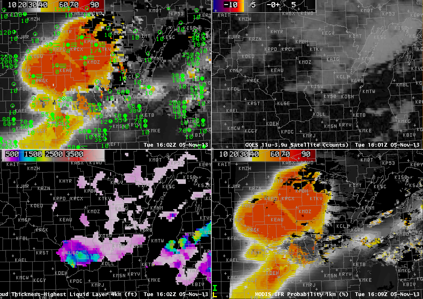
GOES-R IFR Probabilities computed from GOES-East (Upper Left), GOES-East Brightness Temperature Differences (10.7 µm – 3.9 µm) (Upper Right), GOES-R Cloud Thickness (Lower Left), GOES-R IFR Probabilities computed from MODIS, or GOES-East Visible Imagery, times as indicated on 29 April 2014 (click to enlarge)

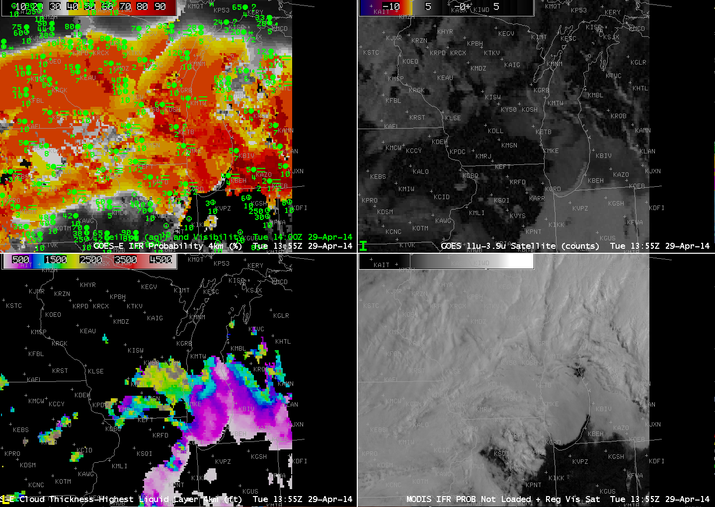
The GOES-R IFR Probability fields computed from GOES-East captured the onset of Lake fog that moved onshore over eastern Wisconsin on April 29th. Multiple cloud layers associated with a strong extratropical cyclone precluded the use of the brightness temperature difference product (the heritage method of detecting fog/low stratus). However, the IFR Probability field aligns well with the reductions in visibility associated with the Lake fog. The character of the IFR Probability field can be used to infer whether of not satellite data predictors are being used. For example, the relatively flat field over southeast Wisconsin at the start of the animation is a region where satellite predictors are not used. The use of satellite predictors generally leads to a pixelated field. A flatter field as over southeast Wisconsin reflects the smoother model fields that are driving the probability field computation.

Cloud thickness is computed in regions where the highest cloud, as seen by the satellite, is a water-based cloud. And that is also usually the region where satellite predictors are used in the computation of IFR Probabilities. Note in the animation above how cloud thickness generally overlays regions of IFR Probability that are pixelated. Cloud thickness is not computed where only model data are used to compute IFR Probabilities. (Cloud thickness is also not computed in the hour or so around sunrise and sunset, during twilight conditions).

The slow northward movement of the fog bank is apparent in the first part of the animation above, from 0615 through 0745 UTC. Note also how the MODIS IFR Probability fields give a very similar solution to the GOES-13-based fields at 0745 UTC. Differences in resolution are apparent over southwest Wisconsin, however, where river valleys are more accurately captured by the MODIS fields.

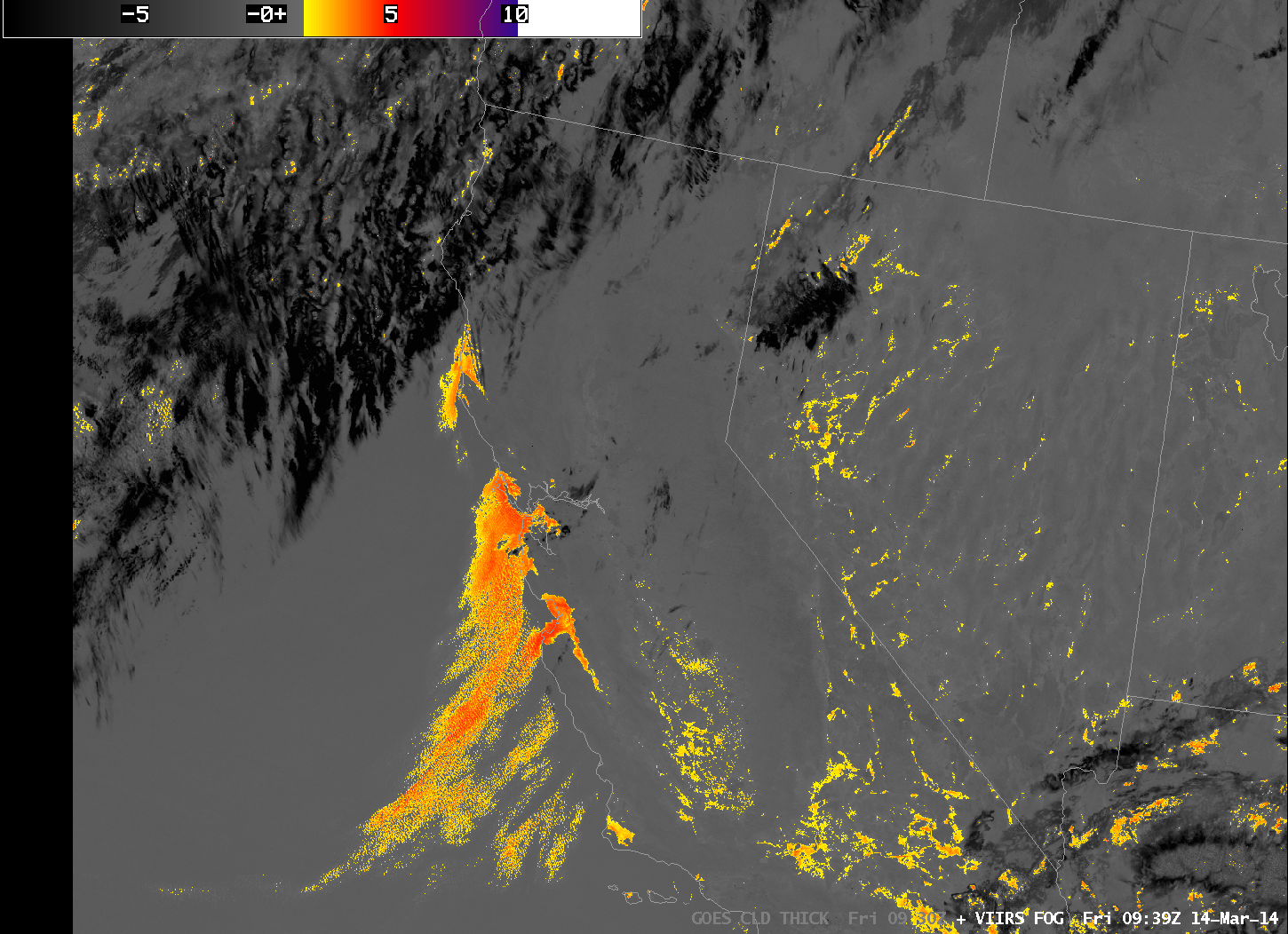
In the visible imagery at the end of the animation (1355 UTC), the rapid saturation of moisture-laden air moving northward from Indiana over the cold waters of southern Lake Michigan is very apparent.

Low clouds and Fog along the West Coast

Low clouds and fog developed along the west coast this morning. From the Monterey (CA) AFD:

FXUS66 KMTR 141143
AFDMTR

AREA FORECAST DISCUSSION
NATIONAL WEATHER SERVICE SAN FRANCISCO BAY AREA
443 AM PDT FRI MAR 14 2014

.SYNOPSIS…AFTER A BIT OF COOLING TODAY…A WARM AND DRY UPPER LEVEL
RIDGE OF HIGH PRESSURE WILL BUILD STRONGLY INTO THE WEST COAST
OVER THE WEEKEND. THIS WILL RESULT IN AFTERNOON TEMPERATURES
REACHING WELL ABOVE SEASONAL NORMS…AND POSSIBLY TO NEAR RECORD
LEVELS FOR THESE DATES. THIS WARM-UP WILL BE SHORT-LIVED HOWEVER…WITH
INCREASED ONSHORE FLOW AND A SIGNIFICANTLY COOLER AIR MASS MOVING
IN ALOFT THE FIRST PART OF NEXT WEEK. DRY CONDITIONS ARE EXPECTED
TO CONTINUE THROUGH MID WEEK…BUT THEN WITH UPPER LEVEL TROUGHING
AND A CHANCE OF RAIN FOR THE OUTER PORTION OF THE FORECAST PERIOD.

&&

.DISCUSSION…AS OF 4:10 AM PDT FRIDAY…THE DRY TAIL END OF A
WEATHER SYSTEM MOVING IN TO THE PACIFIC NORTHWEST IS APPROACHING
OUR DISTRICT…AND RESULTING IN ENHANCEMENT OF THE MARINE LAYER
AND A RETURN OF THE MARINE STRATUS. LATEST GOES FOG PRODUCT
IMAGERY…AND IN RATHER SPECTACULAR DETAIL JUST REC’D SUOMI VIIRS
NIGHTTIME HIGH RES VISUAL IMAGE…SHOW COVERAGE ALONG MUCH OF THE
COAST FROM PT REYES SOUTH TO THE VICINITY OF THE MONTEREY
PENINSULA…AND A BROAD SWATH EXTENDING INLAND ACROSS SAN
FRANCISCO AND THROUGH THE GOLDEN GATE TO THE EAST BAY. LATEST
BODEGA BAY AND FT ORD PROFILER DATA INDICATE A MARINE LAYER DEPTH
OF ABOUT 1300 FT. SOME THIN HIGH CLOUDS ARE ALSO PASSING THROUGH ABOVE.

NAM MODEL AND IN-HOUSE LOCAL WRF MODEL BOUNDARY LAYER RH OUTPUT
BOTH INDICATE STRATUS SHOULD GENERALLY CLEAR BY MIDDAY…EXCEPT
ALONG THE SAN MATEO COAST AND IN THE VICINITY OF THE MONTEREY
PENINSULA. EXPECT AFTERNOON HIGHS TO BE AROUND 3 TO 5 DEGS COOLER
THAN ON THURSDAY…BUT STILL WELL ABOVE SEASONAL NORMS ESPECIALLY
INLAND.

GOES_IFR_PROB_20140314loop

GOES-R IFR Probabilities computed from GOES-15 (Upper Left), GOES-West Brightness Temperature Differences (10.7 µm – 3.9 µm) (Upper Right), GOES-R Cloud Thickness (Lower Left), Suomi/NPP Day/Night Band (Lower Right), all hourly times as indicated (click to enlarge)

The animation of satellite and satellite-derived fields, above, shows how the GOES-R and GOES-West fields depicted the development of the low clouds. Note how the brightness temperature difference fields over CA and NV throughout the animation have a speckled appearance. These positive signals are due not to the presence of fog/low clouds but rather to differences in emissivity properties of the dry land. Near the end of the animation, high clouds are widespread over northern California. For such cases, the brightness temperature difference product provides little information about low-level clouds. However, the GOES-R IFR Probability field, because it blends together information from satellite and from Rapid Refresh does provide a signal under clouds. It is a much smoother signal because it does vary from one satellite pixel to the next, and the Probability values are smaller because satellite predictors cannot be used in the algorithm.

The AFD above notes the Day/Night band, and also the depth of the marine stratus. The toggle of Cloud Thickness, Day/Night Band, and brightness temperature difference, below (useful to distinguish white clouds from white city lights!), shows a nice overlap between the GOES-R product and the clouds detected at high resolution by Suomi/NPP. Cloud thickness is around 1150 feet at Bodega Bay, and closer to 1250 feet at Fort Ord, in good agreement with the profile data cited.

VIIRS_DNB__REF_GOES_CLD_THICK_20140314_09

Toggle of GOES-R Cloud Thickness, Suomi/NPP Brightness Temperature Difference and Day/Night Band (click to enlarge)

Dense fog on the East Coast

VIIRS_DNB_FOG_20140115toggle

GOES-East IFR Probabilities and surface plots of visibilities/ceilings at 0615 UTC 15 January (Upper Left), GOES-East Brightness Temperature Difference (10.7 µm – 3.9 µm), 0615 UTC 15 January (Upper Right), GOES-R Cloud Thickness, 0615 UTC 15 January (Lower Left), and Suomi/NPP Day/Night Band and Brightness Temperature Difference toggle (11.35 µm – 3.74 µm), 0605 UTC 15 January (Lower Right)(click image to enlarge)

The image above documents the GOES-R IFR Probability field during a fog event over the East Coast. Note how the IFR Probability field shows more horizontal uniformity than the traditional brightness temperature difference field over eastern Pennsylvania (where IFR conditions are reported). For example, both Selinsgrove along the Susquehanna and Reading in south-central Pennsylvania report IFR conditions in regions where the IFR Probability field has a strong return, but where the brightness temperature difference field’s diagnosis is less certain.

The Suomi/NPP field demonstrates the importance of higher resolution from polar orbiting satellites. Both the Day/Night Band and the brightness temperature difference fields suggest the presence of river valley fog over the West Branch of the Susquehanna and its many tributaries in central Pennsylvania. This continues at 0743 UTC, below, when Suomi/NPP’s subsequent overpass also viewed the Susquehanna valley. At both times, the river fog is too small-scale to be detected with GOES-13’s nominal 4-km pixel size.

VIIRS_DNB_FOG_20140115toggle

GOES-East IFR Probabilities and surface plots of visibilities/ceilings at 0745 UTC 15 January (Upper Left), GOES-East Brightness Temperature Difference (10.7 µm – 3.9 µm), 0745 UTC 15 January (Upper Right), GOES-R Cloud Thickness, 0745 UTC 15 January (Lower Left), and Suomi/NPP Day/Night Band and Brightness Temperature Difference toggle (11.35 µm – 3.74 µm), 0743 UTC 15 January (Lower Right)(click image to enlarge)

The animation of the fields, below, done to demonstrate the importance of GOES-13’s temporal resolution, shows how the GOES-R IFR Probability field accurately captures the extent of the fog, even as the sun rises and causes the sign of the brightness temperature difference to flip. The traditional brightness temperature difference field has difficulty both in maintaining a signal through sunrise, and it diagnosing the region of fog/low stratus over northcentral Pennsylvania in and around the Poconos and in the Susquehanna River valley. The IFR Probability field has a minimum over/around Mt. Pocono, where IFR conditions are not observed until close to sunrise. IFR probabilities are small over Altoona, where the brightness temperature difference field shows a strong signal developing late at night (and where observations suggest an elevated stratus deck). In this region, although the satellite suggests fog might be present, model conditions do not agree, and IFR Probabilities are correctly minimized.

GOES-R Cloud thickness suggests that the thickest blanket of fog is over New Jersey. This diagnosis continues up through the twilight conditions of sunrise, at which point Cloud thicknesses are no longer diagnosed.

GOES_IFR_PROB_20140115loop

GOES-East IFR Probabilities and surface plots of visibilities/ceilings (Upper Left), GOES-East Brightness Temperature Difference (10.7 µm – 3.9 µm) (Upper Right), GOES-R Cloud Thickness (Lower Left), and GOES-East Water Vapor (6.7 µm), all times as indicated (Lower Right)(click image to enlarge)

IFR Conditions over Oklahoma and Kansas

GOES_IFR_PROB_20140108_2345

GOES-R IFR Probabilities from GOES-13 (upper left), GOES-13 Brightness Temperature Difference (10.7 µm – 3.9 µm) Fields (upper right), GOES-R Cloud Thickness from GOES-13 (lower left), Suomi/NPP Day/Night Band (lower right), ~2345 UTC 8 January 2014 (click image to enlarge)

IFR Conditions developed over portions of Kansas and Oklahoma (and adjacent states) overnight. How did the GOES-R IFR Probability field diagnose the development of this event? At ~0000 UTC, the traditional method of low stratus/fog detection (Brightness Temperature Difference) showed two regions over the Plains, one centered over Oklahoma, and one over the Kansas/Nebraska border. IFR Probabilities at the same time covered a smaller area; Wichita in particular had low IFR Probabilities despite a brightness temperature difference signal, and Wichita did not report IFR conditions at the time.

Note that high clouds are also present in the Brightness Temperature Difference field over western Kansas, the panhandles of Texas and Oklahoma, and New Mexico. In the enhancement used, high clouds are depicted as dark greys.

GOES_IFR_PROB_20140109_0202

As above, but at 0202 UTC 9 January 2014 (click image to enlarge)

By 0200 UTC (above), the high clouds have moved over parts of Oklahoma and Kansas. Consequently, there are regions over central Oklahoma and south-central Kansas where the brightness temperature difference field is not useful in detecting low stratus/fog that is occurring. The IFR Probability fields suggest the presence of low clouds despite the lack of satellite data because the IFR Probability Field also uses output from the Rapid Refresh Model that suggests saturation is occurring in those regions. Model data are also used where satellite data suggest low clouds/stratus are present to delineate where surface ceilings/visibilities are congruent with IFR conditions. As at 2345 UTC, Wichita is not reporting IFR conditions, although the brightness temperature difference field suggests IFR conditions might exist. The IFR Probability field correctly shows low values there.

GOES_IFR_PROB_20140109_0802_VIIRS

As above, but at 0802 UTC 9 January 2014. Suomi/NPP data is a toggle of Day/Night band and 11.35 µm – 3.74 µm brightness temperature difference (click image to enlarge)

By 0802 UTC, high clouds have overspread much of Oklahoma, yet IFR conditions are occurring at several locations. IFR probabilities nicely depict the widespread nature of this IFR event. Probabilities are reduced in regions where high clouds are present because the algorithm cannot use satellite predictors of low clouds/stratus there. Both the Day/Night band and the brightness temperature difference field give information about the top of the cloud deck — it’s hard to infer how the cloud base is behaving. The addition of Rapid Refresh model information on low-level saturation helps better define where IFR conditions are present.

GOES_IFR_PROB_20140109_0945_VIIRS

As above, but at 0945 UTC 9 January 2014. Suomi/NPP data is a toggle of Day/Night band and 11.35 µm – 3.74 µm brightness temperature difference (click image to enlarge)

By 0945 UTC, above, the time of the next Suomi/NPP overpass, the high clouds have started to move eastward out of Oklahoma. Consequently, satellite data can be used as one of the predictors in the IFR probability field, and IFR Probabilities over Oklahoma increase. By 1215 UTC (below), higher clouds have east out of the domain, and IFR Probabilities are high over the region of reduced ceilings/visibilities over Oklahoma. The algorithm continues to show lower probabilities in regions over Kansas where the Brightness temperature difference signals the presence of low stratus/fog but where IFR conditions are not present. Again, this is because the Rapid Refresh model in those regions is not showing low-level saturation.

GOES_IFR_PROB_20140109_1215

As above, but at 1215 UTC 9 January 2014 (click image to enlarge)

Note in the imagery above how the presence of high clouds affects the GOES-R Cloud Thickness. If the highest cloud detected is ice-based, no cloud thickness field is computed. GOES-R Cloud Thickness is the estimated thickness of the highest water-based cloud detected. If ice clouds are present, the highest water-based cloud cannot be detected by the satellite. Cloud Thickness is also not computed during twilight conditions. Those occurred just before the first image, top, and about an hour after the last image, above.

The influence of high clouds

GOES_IFR_PROB_20131216_0700

GOES-R IFR Probabilities from GOES-15 (upper left), GOES-15 and GOES-13 Brightness Temperature Difference (10.7 µm – 3.9 µm) Fields (upper right), GOES-R Cloud Thickness from GOES-15 (lower left), GOES-13 and GOES-15 6.7 µm enhanced water vapor imagery (lower right), all at ~0700 UTC 16 December 2013 (click image to enlarge)

High clouds in the atmosphere limit the ability of satellites to sense the presence of low clouds, as this example from December 16 2013 on the coast of Oregon demonstrates. Both the brightness temperature difference product and the water vapor imagery show signatures that accompany high cirrus. When cirrus is present, the brightness temperature difference field cannot be used to isolate regions of fog and low stratus because the satellite is detecting radiation from the highest emitting surface (the cirrus) not the fog/low stratus beneath. The IFR Probability field, however, uses both cloud information and Rapid Refresh Data, and the model data can fill in regions where satellites give no useful information, such as the lower Columbia River Valley around Astoria. Because satellite data are not used as a predictor, probabilities are lower. Remember how the presence of high clouds affects things when you interpret the IFR Probability fields.

GOES-R Cloud Thickness is not computed under high clouds. The GOES-R Cloud Thickness is the thickness of the highest water-based cloud deck. If a cirrus deck is present, or if twilight conditions are present, GOES-R Cloud Thickness is not computed.

Fog Detection under Cirrus

GOES_IFR_PROB_20131202loop

GOES-R IFR Probabilities from GOES-13 (Upper Left), GOES-13 Brightness Temperature Difference Product (10.7 µm – 3.9 µm) (Upper Right), GOES-R Cloud Thickness from GOES-13 (Lower Left), MODIS-based IFR Probabilities (Lower Right), Times as indicated (click image to enlarge)

Dense Fog developed over the southern Plains overnight, and the case demonstrates how the Fused data product is able to give a useful signal of IFR probabilities even in regions where high clouds preclude the detection of low clouds by satellite. The fog was widespread and dense enough to warrant Dense Fog Advisories from Tulsa, Norman and Topeka forecast offices. See below, for example.

000
FXUS64 KTSA 020953
AFDTSA

AREA FORECAST DISCUSSION
NATIONAL WEATHER SERVICE TULSA OK
353 AM CST MON DEC 2 2013

.DISCUSSION…
DENSE FOG CONTINUES THIS MORNING ACROSS MUCH OF THE CWA. GIVEN THE
TIME OF YEAR /LOW SUN ANGLE/ AND THE FACT THAT SOME HIGH CLOUDS ARE
STREAMING INTO THE AREA FROM THE NW /REDUCED INSOLATION AND
DELAYED MIXING/…THINK IT MAY TAKE A LITTLE LONGER THAN
PREVIOUSLY EXPECTED TO GET RID OF THE FOG. WE HAVE EXTENDED THE
DENSE FOG ADVISORY UNTIL 11 AM. ONCE THE FOG BURNS OFF…SHOULD
BE A PLEASANT DAY WITH UNSEASONABLY WARM TEMPS AND FAIRLY LIGHT
WIND. COULD BE SOME MORE FOG TUESDAY MORNING IN SOME PLACES BUT A
LITTLE MORE WIND MAY KEEP IT FROM GETTING AS DENSE AND AS
WIDESPREAD AS IT IS THIS MORNING. SLIGHTLY WARMER TEMPS IN STORE
TUESDAY WITH SOME PLACES LIKELY IN THE 70S. WARM AND WINDY
CONDITIONS WILL RESULT IN AN INCREASING FIRE WEATHER CONCERN.

Satellite detection of this fog event was constrained by the presence of two upper-level cloud decks. At the beginning of the animation, above, high clouds associated with the subtropical jet are over the southern quarter of the domain plotted. These high clouds quickly shift southward, and the region in the brightness temperature difference product that is consistent with detection of fog/low stratus (that is, low water-based clouds) expands to the south (surface observations suggest the low stratus clouds were present earlier, but masked by the higher clouds). Later in the animation, high clouds sag southward into the northern part of the domain. When this happens, low stratus/fog (indicated in observations by IFR conditions) are not detected by GOES because the higher ice clouds block the view of the scene. However, the IFR Probability fields that use both satellite data and output from the Rapid Refresh Model continue to depict a likely region (confirmed by the observations) of reduced visibilities. IFR Probabilities do drop, of course, as satellite data cannot be used to confirm the presence of low clouds. Knowledge of why the probabilities drop is vital to the interpretation of the field: You have to know that the high clouds are present, either by looking at the satellite data, or by understanding that the character of the IFR Probability field changes to one that is less pixelated when satellite data cannot be included because of ice clouds above the low stratus deck.

GOES_IFR_PROB_20131202_0802

GOES-R IFR Probabilities from GOES-13 (Upper Left), GOES-13 Brightness Temperature Difference Product (10.7 µm – 3.9 µm) (Upper Right), GOES-R Cloud Thickness from GOES-13 (Lower Left), MODIS-based IFR Probabilities (Lower Right), Times near 0802 UTC as indicated (click image to enlarge)

For a large-scale event like this, MODIS-based IFR Probabilities overlap well with GOES-Based IFR Probabilities, as shown in the image above. In cases like this sometimes individual river valleys will show up with slightly elevated IFR Probabilities (or cloud thicknesses).

The GOES-R Cloud Thickness field is computed for the highest water-based cloud detected (during non-twilight conditions — that is, not during the hour or so surrounding sunrise and sunset). Note how well the thickest clouds — over northeast OK, surrounding Tulsa — correlate with the strongest Brightness Temperature Difference, both in GOES and in Suomi/NPP data (below). Note also how the Cloud Thickness field is not computed in regions where higher ice-based clouds are present.

VIIRS_FOG_20131202_0808

GOES-R IFR Probabilities from GOES-13 (Upper Left), GOES-13 Brightness Temperature Difference Product (10.7 µm – 3.9 µm) (Upper Right), GOES-R Cloud Thickness from GOES-13 (Lower Left), Suomi/NPP Brightness Temperature Difference from VIIRS (10.35 µm – 3.74 µm) (Lower Right), Times near 0802 UTC as indicated (click image to enlarge)

Cloud Thickness can be used to predict the time of fog dissipation, using this scatterplot/relationship. If sun angle is limited by the season, or if solar insolation is limited by higher clouds, you might adjust the first guess for dissipation to a later time.

Fog in eastern Washington

GOES_IFR_PROB_20131115loop

GOES-15-based GOES-R IFR Probabilities (Upper Left), GOES-15 Brightness Temperature Difference Product (10.7 µm – 3.9 µm) (Upper Right), GOES-R Cloud Thickness from GOES-15 (Lower Left), Suomi/NPP Brightness Temperature Difference and GOES-15 Visible data (Lower Right), all times as indicated (click image to enlarge)

The evolution of GOES-R IFR Probability fields showed an expected relationship between where Fog and Low stratus caused IFR Conditions and where IFR Probability was highest. The hourly animation, above, shows very high IFR Probabilities in and around Spokane in concert with IFR conditions that are observed. The Brightness Temperature Difference product, upper right, shows a strong signal there as well, but the positive signal extends to regions where IFR conditions are not observed: for example, over western Montana near Missoula. GOES-R IFR Probability fields thus are refining the signal in the brightness temperature difference field; the Rapid Refresh Model output allows the IFR Probability field algorithm to distinguish between fog/low stratus and mid-level stratus.

Later in the animation, IFR Probabilities decrease around Spokane as high-level clouds move in. Because these high clouds obscure the satellite view of low- and mid-level clouds, satellite information is not included in the computation of IFR Probabilities and Probabilities are lower. At the end of the animation, during the day, probabilities increase. Use of the visible data as a cloud-clearing product leads to higher probabilities (because there is more confidence that the cloud is actually present).

Note that Cloud Thickness is only computed in regions of low clouds that are comprised of water droplets. When high clouds are present, cloud thickness is not computed. In addition, cloud thickness is not computed during twilight conditions on either side of sunrise and sunset. Those restrictions show up plainly in the cloud thickness field in the animation.

How accurate are GOES-R Cloud Thickness Fields?

GOES_IFR_PROB_20131111_1145

GOES-13-based GOES-R IFR Probabilities (Upper Left), GOES-13 Brightness Temperature Difference Product (10.7 µm – 3.9 µm) (Upper Right), GOES-R Cloud Thickness from GOES-East (Lower Left), GOES-R Cloud Thickness from GOES-West (Lower Right), all times as indicated (click image to enlarge)

GOES-R IFR Probabilities over the Central Plains from just before sunrise on 11 November 2013 are displayed above. The IFR Probabilities accurately depict the region of lower stratus and fog with reduced visibilities, separating that region from the mid-level stratus over eastern Kansas and western Missouri. In contrast the brightness temperature difference field (10.7 µm – 3.9 µm) highlights the entire region as one of interest.

The GOES-R Cloud Thickness from GOES-East (bottom left) and from GOES-West (bottom right) show cloud thickness over Dodge City at just under 1200 feet. Note that the values computed with GOES-West are somewhat larger because of the oblique view angle from GOES-West. The 1200 UTC sounding from Dodge City, below, shows a fog/stratus deck from the surface (928 mb, 2652 feet ASL) to 880 mb (4075 feet ASL), a thickness of 1423 feet. Given that the sounding is not saturated at the surface, that 1423 foot thickness is likely a slight overestimate. It is very close to the GOES-R Cloud Thickness estimate of 1200 feet, however.

KDDC_20131111_1200

1200 UTC Sounding at Dodge City, Kansas, 11 November 2013 (click image to enlarge)

Fog and Stratus in one scene: What should be highlighted?

GOES_IFR_PROB_20131105loop

GOES-13-based GOES-R IFR Probabilities (Upper Left), GOES-13 Brightness Temperature Difference Product (10.7 µm – 3.9 µm) (Upper Right), GOES-R Cloud Thickness (Lower Left), Suomi-NPP Day/Night band (Lower Right), all times as indicated (click image to enlarge)

Dense fog developed over Western Wisconsin before sunrise on 5 November 2013. The animation above shows the development of high IFR probabilities in that region as a mid-level stratus deck shifts off to the east. Cloud thicknesses just before sunrise reach 1100 feet over portions of Wisconsin; according to this plot, fog should persist for at least 4 hours after sunrise. This was the case. Fog dissipated shortly after 1700 UTC.

This case shows a benefit of the GOES-R IFR Probability field: it accurately discerns the difference between low stratus/fog (that develops over western Wisconsin) and mid-level stratus (retreating to the east over central and eastern Wisconsin during the animation). Mid-level stratus is normally not a transportation concern whereas low clouds/fog most definitely are; in this case, dense fog advisories were issued by the Lacrosse, WI, WFO (ARX). At the beginning of the animation, widespread mid-level stratus is indicated (IFR conditions are not reported). As the night progresses, IFR Probabilities increase in regions where IFR conditions start to be reported. (A brightness temperature signal in GOES also develops in this region).

VIIRSDNB_FOG_20131105_0815

As above, but at 0815 UTC. The lower right image toggles between the Day/Night Band and the Brightness Temperature Difference (11.45 µm – 3.74 µm) from Suomi/NPP (click image to enlarge)

Suomi/NPP VIIRS viewed this scene shortly after 0815 UTC, and that imagery is above. Both the Day/Night band and the Brightness Temperature Difference fields (11.45 µm – 3.74 µm) are shown as a toggle. The mid-level stratus at 0815 is readily apparent. The developing fog over river valleys in western Wisconsin shows plainly in the brightness temperature difference field, but less so in the day/night band with scant lunar illumination.

MODIS_IFR_PROB_20131105loop

GOES-13-based GOES-R IFR Probabilities (Upper Left), GOES-13 Brightness Temperature Difference Product (10.7 µm – 3.9 µm) (Upper Right), GOES-R Cloud Thickness (Lower Left), MODIS-based IFR Probabilities (Lower Right), all times as indicated (click image to animate)

MODIS data from Terra and Aqua is also used to produce IFR Probabilities, and those data are shown above, for three times: 0413 UTC, 0823 UTC and 1609 UTC. Patterns in the MODIS IFR Probability are similar to those in GOES, but small-scale features such as river valleys are much more apparent. Note that by 1609 UTC, higher clouds have overspread western Wisconsin in advance of an approaching mid-latitude cyclone; thus, the GOES and MODIS IFR Probabilities both are flat fields that are mostly based on Rapid Refresh data. Nevertheless, they both depict the region of IFR conditions over western Wisconsin that is surrounded by better visibilities and higher ceilings. Recall that GOES-R cloud thickness is not computed where high clouds are present.

Stratus/Low Clouds with developing Storms on the Plains

GOES_IFR_PROB_20131029loop

GOES-13-based GOES-R IFR Probabilities (Upper Left), GOES-13 Brightness Temperature Difference Product (10.7 µm – 3.9 µm) (Upper Right), GOES-R Cloud Thickness (Lower Left), Suomi-NPP Day/Night band (Lower Right), all times as indicated (click image to animate)

The ongoing change of seasons means that stronger large-scale weather systems are more likely. When something like a Colorado Cyclone moves from the Rockies and emerges into the central part of USA, it brings multiple cloud layers with it, and those many cloud layers make detection of fog and low stratus difficult. The animation above shows GOES-R IFR Probabilities and Cloud Thicknesses as well as the color-enhanced GOES-13 Brightness Temperature Difference (BTD) field. Note the characteristic signal in the BTD field of jet-level cirrus over Kansas. In these regions, BTD fields cannot be used to diagnose regions of low-level clouds because the upper-level clouds block the satellite view of lower clouds.

IFR Probability does have a signal over Kansas, however (where IFR conditions are present — see the animation below). Rapid Refresh data are being used under the cirrus to diagnose the probability of IFR conditions. Thus, IFR Probability fields are filled in under regions of high cirrus. Because only model data are being used to diagnose IFR Probability fields over central and southern Kansas, the characteristic of the field is different. Where satellite and model data are used, as over western Nebraska, the IFR Probability field has a pixelated appearance; where only model data are used, as over southern Kansas, the IFR probability field has a very smooth appearance. In model-only regions, in addition, IFR Probabilities are smaller because the number of predictors available to the algorithm is smaller.

The BTD field highlights regions in eastern Nebraska as having water-based clouds? Are these clouds causing low ceilings and reduced visibilities? No, and IFR probabilities in that region are low. In this region, Rapid Refresh data do not show low-level saturation, and thus the IFR Probabilities are correctly small, despite the strong satellite signal.

GOES_IFR_PROB_20131029withobs_loop

GOES-13-based GOES-R IFR Probabilities and surface visibilities/ceilings, all times as indicated (click image to enlarge)

GOES-R Cloud Thickness, shown at top, is only computed in regions where the highest cloud detected by the satellite is water-based; the algorithm considers includes information from a cloud-typing algorithm, and if clouds are ice phase (or mixed phase) as is likely in the case of jet stream cirrus, cloud thickness is not computed. (Cloud Thickness is also not computed during times of twilight — that is, an hour or so on either side of sunrise and sunset).

GOES_IFR_PROB_20131029_straylightloop

As above, but for a case of Stray Light, all times as indicated (click image to enlarge)

There are still cases at night when Stray Light will contaminate/enhance the 3.9 µm signal on GOES-13, and this contamination can propagate into the GOES-R IFR Probability of Cloud Thickness Fields. In this case, only the Cloud Thickness Fields are affected (below); Cloud thickness jumps about 500 feet for one time period (0415 UTC).