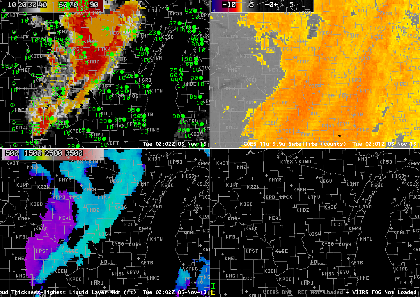
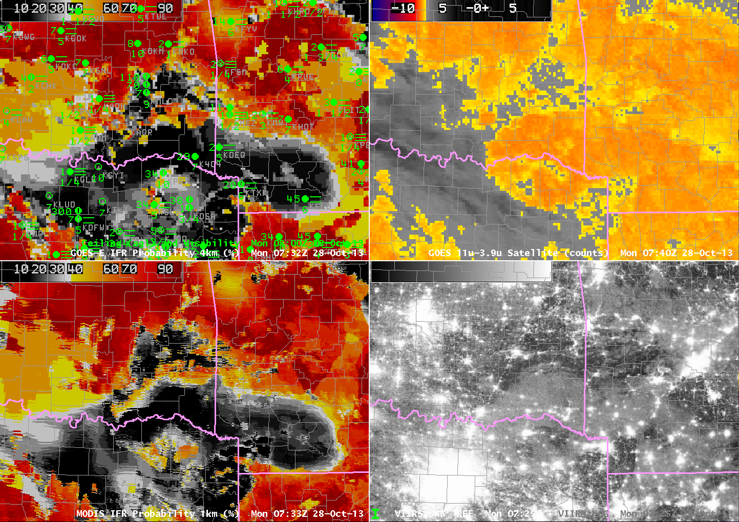
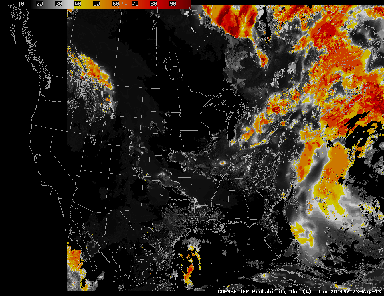
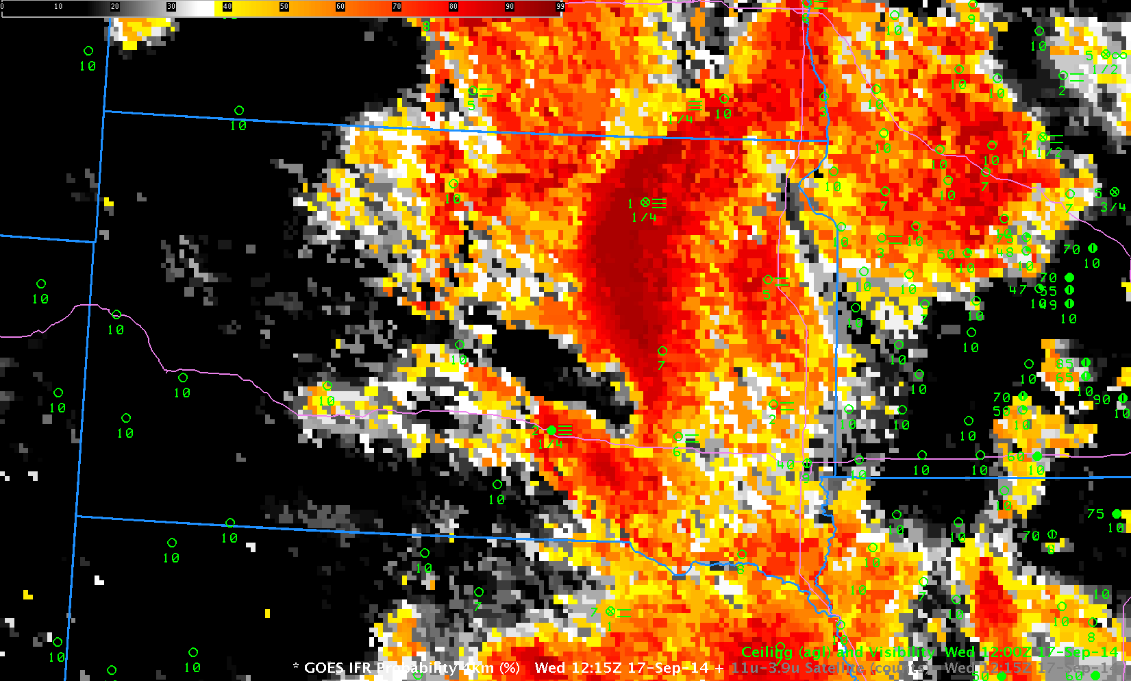
GOES-13-based GOES-R IFR Probabilities (Upper Left), GOES-13 Brightness Temperature Difference Product (10.7 µm – 3.9 µm) (Upper Right), GOES-R Cloud Thickness (Lower Left), Suomi-NPP Day/Night band (Lower Right), all times as indicated (click image to enlarge)
Dense fog developed over Western Wisconsin before sunrise on 5 November 2013. The animation above shows the development of high IFR probabilities in that region as a mid-level stratus deck shifts off to the east. Cloud thicknesses just before sunrise reach 1100 feet over portions of Wisconsin; according to this plot, fog should persist for at least 4 hours after sunrise. This was the case. Fog dissipated shortly after 1700 UTC.
This case shows a benefit of the GOES-R IFR Probability field: it accurately discerns the difference between low stratus/fog (that develops over western Wisconsin) and mid-level stratus (retreating to the east over central and eastern Wisconsin during the animation). Mid-level stratus is normally not a transportation concern whereas low clouds/fog most definitely are; in this case, dense fog advisories were issued by the Lacrosse, WI, WFO (ARX). At the beginning of the animation, widespread mid-level stratus is indicated (IFR conditions are not reported). As the night progresses, IFR Probabilities increase in regions where IFR conditions start to be reported. (A brightness temperature signal in GOES also develops in this region).
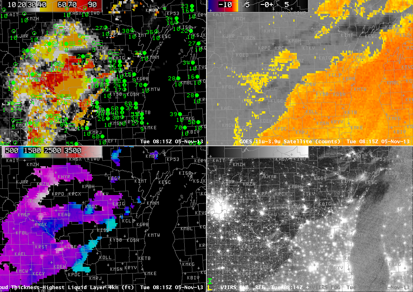
As above, but at 0815 UTC. The lower right image toggles between the Day/Night Band and the Brightness Temperature Difference (11.45 µm – 3.74 µm) from Suomi/NPP (click image to enlarge)
Suomi/NPP VIIRS viewed this scene shortly after 0815 UTC, and that imagery is above. Both the Day/Night band and the Brightness Temperature Difference fields (11.45 µm – 3.74 µm) are shown as a toggle. The mid-level stratus at 0815 is readily apparent. The developing fog over river valleys in western Wisconsin shows plainly in the brightness temperature difference field, but less so in the day/night band with scant lunar illumination.
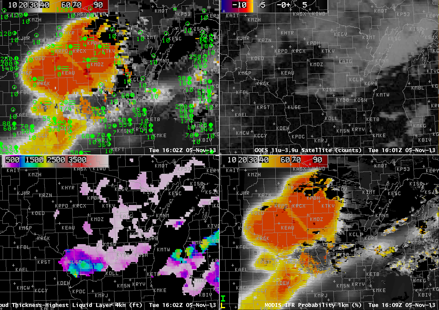
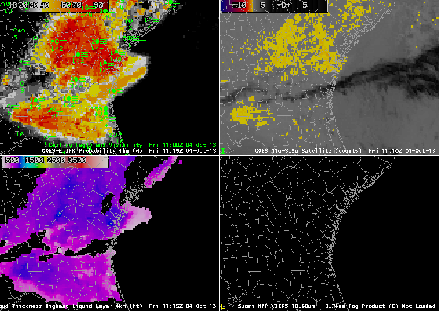
GOES-13-based GOES-R IFR Probabilities (Upper Left), GOES-13 Brightness Temperature Difference Product (10.7 µm – 3.9 µm) (Upper Right), GOES-R Cloud Thickness (Lower Left), MODIS-based IFR Probabilities (Lower Right), all times as indicated (click image to animate)
MODIS data from Terra and Aqua is also used to produce IFR Probabilities, and those data are shown above, for three times: 0413 UTC, 0823 UTC and 1609 UTC. Patterns in the MODIS IFR Probability are similar to those in GOES, but small-scale features such as river valleys are much more apparent. Note that by 1609 UTC, higher clouds have overspread western Wisconsin in advance of an approaching mid-latitude cyclone; thus, the GOES and MODIS IFR Probabilities both are flat fields that are mostly based on Rapid Refresh data. Nevertheless, they both depict the region of IFR conditions over western Wisconsin that is surrounded by better visibilities and higher ceilings. Recall that GOES-R cloud thickness is not computed where high clouds are present.


